Tutorial nsforesting
This tutorial is for running NS-Forest for generating marker combinations that best classify clusters.
Setting up environment
[1]:
import sys
import os
code_folder = "C:/Users/bpeng/OneDrive - J. Craig Venter Institute/Documents/Github/NSForest"
sys.path.insert(0, os.path.abspath(code_folder))
import numpy as np
import pandas as pd
import scanpy as sc
import anndata as ad
import matplotlib.pyplot as plt
import plotly.io as pio
pio.renderers.default = "notebook"
import nsforest as ns
from nsforest import utils
Data Exploration
Loading h5ad AnnData file
[2]:
data_folder = "../demo_data/"
file = data_folder + "adata_layer1.h5ad"
adata = sc.read_h5ad(file)
adata
[2]:
AnnData object with n_obs × n_vars = 871 × 16497
    obs: 'cluster'
Defining cluster_header as cell type annotation.
Note: Some datasets have multiple annotations per sample (ex. “broad_cell_type” and “granular_cell_type”). NS-Forest can be run on multiple cluster_header’s. Combining the parent and child markers may improve classification results.
[3]:
cluster_header = "cluster"
Defining output_folder for saving results
[4]:
output_folder = "../outputs_layer1/"
Looking at sample labels
[5]:
adata.obs_names
[5]:
Index(['A01_1_Nuclei_NeuNP_H200_1025_MTG_layer1_BCH9',
       'A01_BCH3_1NeuNP_H200.1030_MTG_Layer_1',
       'A02_BCH1_1NeuNP_H200.1025_MTG_layer_1',
       'A03_1_Nuclei_NeuNP_H200_1025_MTG_layer1_BCH9',
       'A04_1_Nuclei_NeuNP_H200_1025_MTG_layer1_BCH9',
       'A04_BCH1_1NeuNP_H200.1025_MTG_layer_1',
       'A04_BCH3_1NeuNP_H200.1030_MTG_Layer_1',
       'A05_1_Nuclei_NeuNP_H200_1025_MTG_layer1_BCH9',
       'A05_BCH1_1NeuNP_H200.1025_MTG_layer_1',
       'A05_BCH3_1NeuNP_H200.1030_MTG_Layer_1',
       ...
       'P09_1_Nuclei_NeuNN_H200_1025_MTG_layer1_BCH7',
       'P09_1_Nuclei_NeuNN_H200_1025_MTG_layer1_BCH9',
       'P09_1_Nuclei_NeuNN_H200_1030_MTG_layer1_BCH8',
       'P09_BCH1_1NeuNN_H200.1025_MTG_layer_1',
       'P10_1_Nuclei_NeuNN_H200_1025_MTG_layer1_BCH6',
       'P10_1_Nuclei_NeuNN_H200_1025_MTG_layer1_BCH9',
       'P10_BCH1_1NeuNN_H200.1025_MTG_layer_1',
       'P11_1_Nuclei_NeuNN_H200_1025_MTG_layer1_BCH7',
       'P11_1_Nuclei_NeuNN_H200_1025_MTG_layer1_BCH9',
       'P11_1_Nuclei_NeuNN_H200_1030_MTG_layer1_BCH8'],
      dtype='object', length=871)
Looking at genes
Note: adata.var_names must be unique. If there is a problem, usually it can be solved by assigning adata.var.index = adata.var["ensembl_id"].
[6]:
adata.var_names
[6]:
Index(['A1CF', 'A2M', 'A2M_AS1', 'A2ML1', 'A2ML1_AS1', 'A2MP1', 'A3GALT2',
       'A4GALT', 'AAAS', 'AACS',
       ...
       'ZUFSP', 'ZW10', 'ZWILCH', 'ZWINT', 'ZXDC', 'ZYG11A', 'ZYG11B', 'ZYX',
       'ZZEF1', 'ZZZ3'],
      dtype='object', length=16497)
Checking cell annotation sizes
Note: Some datasets are too large and need to be downsampled to be run through the pipeline. When downsampling, be sure to have all the granular cluster annotations represented.
[7]:
pd.DataFrame(adata.obs[cluster_header].value_counts()).reset_index()
[7]:
| cluster | count | |
|---|---|---|
| 0 | e1_e299_SLC17A7_L5b_Cdh13 | 299 |
| 1 | i1_i90_COL5A2_Ndnf_Car4 | 90 |
| 2 | i2_i77_LHX6_Sst_Cbln4 | 77 |
| 3 | i3_i56_BAGE2_Ndnf_Cxcl14 | 56 |
| 4 | i4_i54_MC4R_Ndnf_Cxcl14 | 54 |
| 5 | g1_g48_GLI3_Astro_Gja1 | 48 |
| 6 | i5_i47_TRPC3_Ndnf_Car4 | 47 |
| 7 | i6_i44_GPR149_Vip_Mybpc1 | 44 |
| 8 | i7_i31_CLMP_Ndnf_Cxcl14 | 31 |
| 9 | g2_g27_APBB1IP_Micro_Ctss | 27 |
| 10 | i8_i27_SNCG_Vip_Mybpc1 | 27 |
| 11 | i9_i22_TAC3_Vip_Mybpc1 | 22 |
| 12 | g3_g18_GPNMB_OPC_Pdgfra | 18 |
| 13 | i10_i16_TSPAN12_Vip_Mybpc1 | 16 |
| 14 | g4_g9_MOG_Oligo_Opalin | 9 |
| 15 | i11_i6_EGF_Vip_Mybpc1 | 6 |
Preprocessing
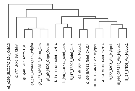
Generating scanpy dendrogram
Note: Only run if there is no pre-defined dendrogram order. This step can still be run with no effects, but the runtime may increase.
Dendrogram order is stored in adata.uns["dendrogram_cluster"]["categories_ordered"].
[8]:
ns.pp.dendrogram(adata, cluster_header, save = True, output_folder = output_folder, outputfilename_suffix = cluster_header)
Saving dendrogram as...
../outputs_layer1/_cluster.png
Calculating cluster medians per gene
Run ns.pp.prep_medians before running NS-Forest.
Note: Do not run if evaluating marker lists. Do not run when generating scanpy plots (e.g. dot plot, violin plot, matrix plot).
[9]:
adata = ns.pp.prep_medians(adata, cluster_header)
adata.varm["medians_cluster"]
Calculating medians per cluster: 100%|██████████| 16/16 [00:01<00:00, 10.19it/s]
Saving medians as adata.varm.medians_cluster
median: 0.0
mean: 1.626
std: 2.49
Only positive genes selected. 11688 positive genes out of 16497 total genes
--- 2.008080244064331 seconds ---
[9]:
| e1_e299_SLC17A7_L5b_Cdh13 | g1_g48_GLI3_Astro_Gja1 | g2_g27_APBB1IP_Micro_Ctss | g3_g18_GPNMB_OPC_Pdgfra | g4_g9_MOG_Oligo_Opalin | i10_i16_TSPAN12_Vip_Mybpc1 | i11_i6_EGF_Vip_Mybpc1 | i1_i90_COL5A2_Ndnf_Car4 | i2_i77_LHX6_Sst_Cbln4 | i3_i56_BAGE2_Ndnf_Cxcl14 | i4_i54_MC4R_Ndnf_Cxcl14 | i5_i47_TRPC3_Ndnf_Car4 | i6_i44_GPR149_Vip_Mybpc1 | i7_i31_CLMP_Ndnf_Cxcl14 | i8_i27_SNCG_Vip_Mybpc1 | i9_i22_TAC3_Vip_Mybpc1 | |
|---|---|---|---|---|---|---|---|---|---|---|---|---|---|---|---|---|
| A2M | 0.000000 | 1.584962 | 8.985842 | 1.000000 | 0.000000 | 0.000000 | 1.792481 | 0.000000 | 0.000000 | 1.000000 | 0.000000 | 1.000000 | 1.292481 | 0.000000 | 1.000000 | 0.500000 |
| A2M_AS1 | 0.000000 | 0.000000 | 3.169925 | 0.000000 | 0.000000 | 0.000000 | 0.000000 | 0.000000 | 0.000000 | 0.000000 | 0.000000 | 0.000000 | 0.000000 | 0.000000 | 0.000000 | 0.000000 |
| A2ML1_AS1 | 4.392317 | 7.832668 | 1.584962 | 4.253898 | 0.000000 | 6.400854 | 3.683161 | 4.522197 | 4.754888 | 2.403677 | 4.321928 | 5.392317 | 4.459432 | 5.209454 | 5.727921 | 5.096147 |
| A2MP1 | 0.000000 | 0.000000 | 0.000000 | 0.000000 | 1.584962 | 0.000000 | 0.000000 | 0.000000 | 0.000000 | 0.000000 | 0.000000 | 0.000000 | 0.000000 | 1.000000 | 1.000000 | 0.000000 |
| AAAS | 0.000000 | 1.292481 | 0.000000 | 0.000000 | 0.000000 | 0.000000 | 0.000000 | 0.000000 | 0.000000 | 0.000000 | 0.000000 | 0.000000 | 0.000000 | 0.000000 | 1.000000 | 0.000000 |
| ... | ... | ... | ... | ... | ... | ... | ... | ... | ... | ... | ... | ... | ... | ... | ... | ... |
| ZYG11A | 0.000000 | 0.000000 | 0.000000 | 0.000000 | 0.000000 | 0.000000 | 1.000000 | 0.000000 | 0.000000 | 0.000000 | 0.000000 | 0.000000 | 0.000000 | 0.000000 | 0.000000 | 0.000000 |
| ZYG11B | 4.857981 | 1.000000 | 1.000000 | 0.000000 | 2.584963 | 3.836213 | 6.346526 | 5.491853 | 3.906891 | 3.064641 | 3.903677 | 5.781360 | 5.584649 | 6.475733 | 5.614710 | 5.931125 |
| ZYX | 3.169925 | 0.000000 | 0.000000 | 0.000000 | 0.000000 | 0.000000 | 0.000000 | 0.000000 | 0.000000 | 0.000000 | 0.000000 | 0.000000 | 0.000000 | 0.000000 | 0.000000 | 0.000000 |
| ZZEF1 | 4.392317 | 1.584962 | 2.321928 | 0.000000 | 1.000000 | 4.215226 | 5.734567 | 3.390680 | 1.584962 | 1.584962 | 2.321928 | 3.169925 | 3.229716 | 4.392317 | 3.584963 | 2.660964 |
| ZZZ3 | 6.303781 | 3.000000 | 1.584962 | 3.435182 | 8.189824 | 5.972722 | 5.985592 | 5.712608 | 4.906890 | 6.374096 | 5.997354 | 6.321928 | 6.169925 | 6.507795 | 5.426265 | 6.492921 |
11688 rows × 16 columns
Calculating binary scores per gene per cluster
Run ns.pp.prep_binary_scores before running NS-Forest. Do not need to run if evaluating marker lists. Do not need to run when generating scanpy plots.
[10]:
adata = ns.pp.prep_binary_scores(adata, cluster_header)
adata.varm["binary_scores_cluster"]
Calculating binary scores per cluster: 100%|██████████| 16/16 [01:13<00:00, 4.62s/it]
Saving binary scores as adata.varm.binary_scores_cluster
median: 0.1
mean: 0.202
std: 0.252
--- 74.26272201538086 seconds ---
[10]:
| e1_e299_SLC17A7_L5b_Cdh13 | g1_g48_GLI3_Astro_Gja1 | g2_g27_APBB1IP_Micro_Ctss | g3_g18_GPNMB_OPC_Pdgfra | g4_g9_MOG_Oligo_Opalin | i10_i16_TSPAN12_Vip_Mybpc1 | i11_i6_EGF_Vip_Mybpc1 | i1_i90_COL5A2_Ndnf_Car4 | i2_i77_LHX6_Sst_Cbln4 | i3_i56_BAGE2_Ndnf_Cxcl14 | i4_i54_MC4R_Ndnf_Cxcl14 | i5_i47_TRPC3_Ndnf_Car4 | i6_i44_GPR149_Vip_Mybpc1 | i7_i31_CLMP_Ndnf_Cxcl14 | i8_i27_SNCG_Vip_Mybpc1 | i9_i22_TAC3_Vip_Mybpc1 | |
|---|---|---|---|---|---|---|---|---|---|---|---|---|---|---|---|---|
| A2M | 0.000000 | 0.623023 | 0.931968 | 0.500000 | 0.000000 | 0.000000 | 0.658949 | 0.000000 | 0.000000 | 0.500000 | 0.000000 | 0.500000 | 0.567888 | 0.000000 | 0.500000 | 0.466667 |
| A2M_AS1 | 0.000000 | 0.000000 | 1.000000 | 0.000000 | 0.000000 | 0.000000 | 0.000000 | 0.000000 | 0.000000 | 0.000000 | 0.000000 | 0.000000 | 0.000000 | 0.000000 | 0.000000 | 0.000000 |
| A2ML1_AS1 | 0.153393 | 0.470567 | 0.066667 | 0.146435 | 0.000000 | 0.352137 | 0.127804 | 0.163316 | 0.184686 | 0.089374 | 0.149377 | 0.247584 | 0.158108 | 0.228193 | 0.283856 | 0.216961 |
| A2MP1 | 0.000000 | 0.000000 | 0.000000 | 0.000000 | 0.915876 | 0.000000 | 0.000000 | 0.000000 | 0.000000 | 0.000000 | 0.000000 | 0.000000 | 0.000000 | 0.866667 | 0.866667 | 0.000000 |
| AAAS | 0.000000 | 0.948420 | 0.000000 | 0.000000 | 0.000000 | 0.000000 | 0.000000 | 0.000000 | 0.000000 | 0.000000 | 0.000000 | 0.000000 | 0.000000 | 0.000000 | 0.933333 | 0.000000 |
| ... | ... | ... | ... | ... | ... | ... | ... | ... | ... | ... | ... | ... | ... | ... | ... | ... |
| ZYG11A | 0.000000 | 0.000000 | 0.000000 | 0.000000 | 0.000000 | 0.000000 | 1.000000 | 0.000000 | 0.000000 | 0.000000 | 0.000000 | 0.000000 | 0.000000 | 0.000000 | 0.000000 | 0.000000 |
| ZYG11B | 0.268527 | 0.066667 | 0.066667 | 0.000000 | 0.148420 | 0.200397 | 0.381241 | 0.306785 | 0.204062 | 0.166928 | 0.203846 | 0.328997 | 0.312765 | 0.393586 | 0.315017 | 0.342573 |
| ZYX | 1.000000 | 0.000000 | 0.000000 | 0.000000 | 0.000000 | 0.000000 | 0.000000 | 0.000000 | 0.000000 | 0.000000 | 0.000000 | 0.000000 | 0.000000 | 0.000000 | 0.000000 | 0.000000 |
| ZZEF1 | 0.401457 | 0.091271 | 0.168100 | 0.000000 | 0.066667 | 0.381913 | 0.541554 | 0.284062 | 0.091271 | 0.091271 | 0.168100 | 0.258675 | 0.264994 | 0.401457 | 0.308410 | 0.206141 |
| ZZZ3 | 0.157010 | 0.031445 | 0.000000 | 0.044353 | 0.347222 | 0.131380 | 0.132101 | 0.119149 | 0.091036 | 0.163913 | 0.132888 | 0.158664 | 0.145953 | 0.178503 | 0.107846 | 0.176774 |
11688 rows × 16 columns
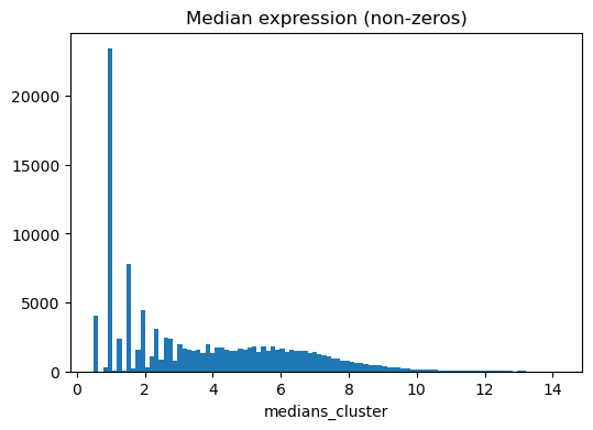
Plotting median and binary score distributions
[11]:
ns.pp.plot_varm(adata, f"medians_{cluster_header}", nonzero = True, save = True, output_folder = output_folder)
Saving adata.varm[medians_cluster] as histogram as...
../outputs_layer1/histogram_medians_cluster.png
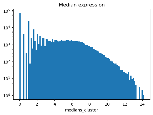
[12]:
ns.pp.plot_varm(adata, f"medians_{cluster_header}", scale = "log", save = True, output_folder = output_folder)
Saving adata.varm[medians_cluster] as histogram as...
../outputs_layer1/histogram_medians_cluster.png
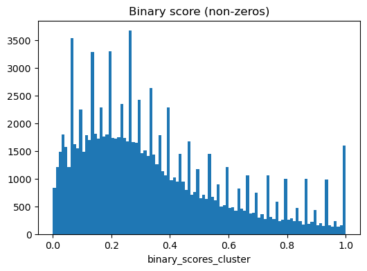
[13]:
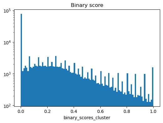
ns.pp.plot_varm(adata, f"binary_scores_{cluster_header}", nonzero = True, save = True, output_folder = output_folder)
Saving adata.varm[binary_scores_cluster] as histogram as...
../outputs_layer1/histogram_binary_scores_cluster.png
[14]:
ns.pp.plot_varm(adata, f"binary_scores_{cluster_header}", scale = "log", save = True, output_folder = output_folder)
Saving adata.varm[binary_scores_cluster] as histogram as...
../outputs_layer1/histogram_binary_scores_cluster.png
Saving preprocessed AnnData as new h5ad
[15]:
filename = file.replace(".h5ad", "_preprocessed.h5ad")
print(f"Saving new anndata object as...\n{filename}")
adata.write_h5ad(filename)
adata
Saving new anndata object as...
../demo_data/adata_layer1_preprocessed.h5ad
[15]:
AnnData object with n_obs × n_vars = 871 × 11688
    obs: 'cluster'
    uns: 'pca', 'dendrogram_cluster'
    obsm: 'X_pca'
    varm: 'PCs', 'medians_cluster', 'binary_scores_cluster'
Running NS-Forest
Note: Do not run NS-Forest if only evaluating input marker lists.
[16]:
outputfilename_prefix = cluster_header
results = ns.nsforesting.NSForest(adata, cluster_header, save_supplementary = True, save = True, output_folder = output_folder, outputfilename_prefix = outputfilename_prefix)
Running NS-Forest version 4.1

Preparing adata...
Pre-selecting genes based on binary scores...
        BinaryFirst_high Threshold (mean + 2 * std): 0.706
        Average number of genes after gene_selection in each cluster: 735.5
Saving number of genes selected per cluster as...
../outputs_layer1/cluster_gene_selection.csv
--- 0.05267214775085449 seconds ---

Number of clusters to evaluate: 16
1 out of 16:
        e1_e299_SLC17A7_L5b_Cdh13
        Pre-selected 1356 genes to feed into Random Forest.
        NSForest-selected markers: ['LINC00507']
        fbeta: 0.96
        precision: 0.978
        recall: 0.893
2 out of 16:
        g1_g48_GLI3_Astro_Gja1
        Pre-selected 583 genes to feed into Random Forest.
        NSForest-selected markers: ['LINC00498']
        fbeta: 0.95
        precision: 1.0
        recall: 0.792
3 out of 16:
        g2_g27_APBB1IP_Micro_Ctss
        Pre-selected 420 genes to feed into Random Forest.
        NSForest-selected markers: ['ADAM28', 'PTPRC']
        fbeta: 0.976
        precision: 1.0
        recall: 0.889
4 out of 16:
        g3_g18_GPNMB_OPC_Pdgfra
        Pre-selected 353 genes to feed into Random Forest.
        NSForest-selected markers: ['GPNMB', 'OLIG2']
        fbeta: 0.862
        precision: 1.0
        recall: 0.556
5 out of 16:
        g4_g9_MOG_Oligo_Opalin
        Pre-selected 571 genes to feed into Random Forest.
        NSForest-selected markers: ['ST18']
        fbeta: 1.0
        precision: 1.0
        recall: 1.0
6 out of 16:
        i10_i16_TSPAN12_Vip_Mybpc1
        Pre-selected 1007 genes to feed into Random Forest.
        NSForest-selected markers: ['TSPAN12', 'CHRNB3']
        fbeta: 0.804
        precision: 0.9
        recall: 0.562
7 out of 16:
        i11_i6_EGF_Vip_Mybpc1
        Pre-selected 1912 genes to feed into Random Forest.
        NSForest-selected markers: ['EGF', 'FBRSL1']
        fbeta: 0.714
        precision: 1.0
        recall: 0.333
8 out of 16:
        i1_i90_COL5A2_Ndnf_Car4
        Pre-selected 238 genes to feed into Random Forest.
        NSForest-selected markers: ['COL5A2', 'BMP6']
        fbeta: 0.908
        precision: 0.97
        recall: 0.722
9 out of 16:
        i2_i77_LHX6_Sst_Cbln4
        Pre-selected 292 genes to feed into Random Forest.
        NSForest-selected markers: ['LHX6']
        fbeta: 0.817
        precision: 0.838
        recall: 0.74
10 out of 16:
        i3_i56_BAGE2_Ndnf_Cxcl14
        Pre-selected 151 genes to feed into Random Forest.
        NSForest-selected markers: ['BAGE2', 'SYT10']
        fbeta: 0.781
        precision: 0.962
        recall: 0.446
11 out of 16:
        i4_i54_MC4R_Ndnf_Cxcl14
        Pre-selected 223 genes to feed into Random Forest.
        NSForest-selected markers: ['ARHGAP36', 'ADAM33']
        fbeta: 0.857
        precision: 0.923
        recall: 0.667
12 out of 16:
        i5_i47_TRPC3_Ndnf_Car4
        Pre-selected 942 genes to feed into Random Forest.
        NSForest-selected markers: ['NTNG1', 'EYA4']
        fbeta: 0.906
        precision: 1.0
        recall: 0.66
13 out of 16:
        i6_i44_GPR149_Vip_Mybpc1
        Pre-selected 377 genes to feed into Random Forest.
        NSForest-selected markers: ['FLT1', 'GPR149']
        fbeta: 0.792
        precision: 1.0
        recall: 0.432
14 out of 16:
        i7_i31_CLMP_Ndnf_Cxcl14
        Pre-selected 1012 genes to feed into Random Forest.
        NSForest-selected markers: ['PAX6', 'TGFBR2']
        fbeta: 0.901
        precision: 1.0
        recall: 0.645
15 out of 16:
        i8_i27_SNCG_Vip_Mybpc1
        Pre-selected 1326 genes to feed into Random Forest.
        NSForest-selected markers: ['SNCG', 'EDNRA']
        fbeta: 0.759
        precision: 0.923
        recall: 0.444
16 out of 16:
        i9_i22_TAC3_Vip_Mybpc1
        Pre-selected 1005 genes to feed into Random Forest.
        NSForest-selected markers: ['BSPRY', 'MCTP2']
        fbeta: 0.69
        precision: 0.889
        recall: 0.364
--- 87.0947813987732 seconds ---

Saving supplementary table as...
../outputs_layer1/cluster_supplementary.csv
Saving markers table as...
../outputs_layer1/cluster_markers.csv
using median
Calculating medians per cluster: 100%|██████████| 16/16 [00:00<00:00, 366.96it/s]
Saving supplementary table as...
../outputs_layer1/cluster_markers_onTarget_supp.csv
Saving supplementary table as...
../outputs_layer1/cluster_markers_onTarget.csv

Saving final results table as...
../outputs_layer1/cluster_results.csv
Saving final results table as...
../outputs_layer1/cluster_results.pkl
[17]:
results
[17]:
| software_version | cluster_header | clusterName | clusterSize | f_score | precision | recall | TN | FP | FN | TP | marker_count | NSForest_markers | binary_genes | onTarget | |
|---|---|---|---|---|---|---|---|---|---|---|---|---|---|---|---|
| 0 | 4.1 | cluster | e1_e299_SLC17A7_L5b_Cdh13 | 299 | 0.959741 | 0.978022 | 0.892977 | 566 | 6 | 32 | 267 | 1 | [LINC00507] | [SLC17A7, LINC00508, TBR1, ANKRD33B, NPTX1, LI... | 0.792614 |
| 1 | 4.1 | cluster | g1_g48_GLI3_Astro_Gja1 | 48 | 0.950000 | 1.000000 | 0.791667 | 823 | 0 | 10 | 38 | 1 | [LINC00498] | [LINC00498, SLC25A18, EMX2OS, FAM189A2, SLC7A1... | 1.000000 |
| 2 | 4.1 | cluster | g2_g27_APBB1IP_Micro_Ctss | 27 | 0.975610 | 1.000000 | 0.888889 | 844 | 0 | 3 | 24 | 2 | [ADAM28, PTPRC] | [ADAM28, PLCG2, INPP5D, PTPRC, CSF2RA, P2RY13,... | 1.000000 |
| 3 | 4.1 | cluster | g3_g18_GPNMB_OPC_Pdgfra | 18 | 0.862069 | 1.000000 | 0.555556 | 853 | 0 | 8 | 10 | 2 | [GPNMB, OLIG2] | [GPNMB, COL20A1, OLIG2, STK32A, KLRC3, KLRC2, ... | 1.000000 |
| 4 | 4.1 | cluster | g4_g9_MOG_Oligo_Opalin | 9 | 1.000000 | 1.000000 | 1.000000 | 862 | 0 | 0 | 9 | 1 | [ST18] | [ST18, MOBP, CNDP1, MOG, CD22, FOLH1, TF, CARN... | 1.000000 |
| 5 | 4.1 | cluster | i10_i16_TSPAN12_Vip_Mybpc1 | 16 | 0.803571 | 0.900000 | 0.562500 | 854 | 1 | 7 | 9 | 2 | [TSPAN12, CHRNB3] | [TSPAN12, TMC5, LINC01539, CHRNB3, FAM46A, ANG... | 0.783762 |
| 6 | 4.1 | cluster | i11_i6_EGF_Vip_Mybpc1 | 6 | 0.714286 | 1.000000 | 0.333333 | 865 | 0 | 4 | 2 | 2 | [EGF, FBRSL1] | [EGF, FZD8, KCNJ2_AS1, FBRSL1, TEKT1, NRG3_AS1... | 1.000000 |
| 7 | 4.1 | cluster | i1_i90_COL5A2_Ndnf_Car4 | 90 | 0.907821 | 0.970149 | 0.722222 | 779 | 2 | 25 | 65 | 2 | [COL5A2, BMP6] | [NMBR, COL5A2, C8ORF4, PAPSS2, TRPC3, BMP6, SS... | 0.642585 |
| 8 | 4.1 | cluster | i2_i77_LHX6_Sst_Cbln4 | 77 | 0.816619 | 0.838235 | 0.740260 | 783 | 11 | 20 | 57 | 1 | [LHX6] | [LHX6, FLT3, TAC1, CALB1, RSPO3, TRBC2, GRIK3,... | 1.000000 |
| 9 | 4.1 | cluster | i3_i56_BAGE2_Ndnf_Cxcl14 | 56 | 0.781250 | 0.961538 | 0.446429 | 814 | 1 | 31 | 25 | 2 | [BAGE2, SYT10] | [BAGE2, SCN5A, GREM2, FAM19A4, SYT10, ARHGAP18... | 0.602383 |
| 10 | 4.1 | cluster | i4_i54_MC4R_Ndnf_Cxcl14 | 54 | 0.857143 | 0.923077 | 0.666667 | 814 | 3 | 18 | 36 | 2 | [ARHGAP36, ADAM33] | [ARHGAP36, MC4R, COBLL1, HLA_B, LINC01435, ADA... | 0.710233 |
| 11 | 4.1 | cluster | i5_i47_TRPC3_Ndnf_Car4 | 47 | 0.906433 | 1.000000 | 0.659574 | 824 | 0 | 16 | 31 | 2 | [NTNG1, EYA4] | [SSTR2, KIRREL, TRPC3, NTNG1, TARID, EYA4, CA2... | 0.380471 |
| 12 | 4.1 | cluster | i6_i44_GPR149_Vip_Mybpc1 | 44 | 0.791667 | 1.000000 | 0.431818 | 827 | 0 | 25 | 19 | 2 | [FLT1, GPR149] | [FLT1, PLCE1_AS1, CXCL12, SLC22A3, PLCE1_AS2, ... | 0.811541 |
| 13 | 4.1 | cluster | i7_i31_CLMP_Ndnf_Cxcl14 | 31 | 0.900901 | 1.000000 | 0.645161 | 840 | 0 | 11 | 20 | 2 | [PAX6, TGFBR2] | [KIAA1644, FGF10, CLMP, PAX6, SP8, TGFBR2, WIF... | 0.547845 |
| 14 | 4.1 | cluster | i8_i27_SNCG_Vip_Mybpc1 | 27 | 0.759494 | 0.923077 | 0.444444 | 843 | 1 | 15 | 12 | 2 | [SNCG, EDNRA] | [SNCG, MMRN2, EDNRA, FBN3, KCNK2, RGS2, SCML4,... | 1.000000 |
| 15 | 4.1 | cluster | i9_i22_TAC3_Vip_Mybpc1 | 22 | 0.689655 | 0.888889 | 0.363636 | 848 | 1 | 14 | 8 | 2 | [BSPRY, MCTP2] | [BSPRY, OFD1P10Y, MCTP2, OFD1P8Y, OFD1P15Y, OF... | 1.000000 |
Plotting scanpy dot plot, violin plot, matrix plot for NS-Forest markers
Note: Assign pre-defined dendrogram order here or use adata.uns["dendrogram_" + cluster_header]["categories_ordered"].
[18]:
to_plot = results.copy()
[19]:
dendrogram = [] # custom dendrogram order
dendrogram = list(adata.uns["dendrogram_" + cluster_header]["categories_ordered"])
to_plot["clusterName"] = to_plot["clusterName"].astype("category")
to_plot["clusterName"] = to_plot["clusterName"].cat.set_categories(dendrogram)
to_plot = to_plot.sort_values("clusterName")
to_plot = to_plot.rename(columns = {"NSForest_markers": "markers"})
[20]:
markers_dict = dict(zip(to_plot["clusterName"], to_plot["markers"]))
markers_dict
[20]:
{'e1_e299_SLC17A7_L5b_Cdh13': ['LINC00507'],
 'i2_i77_LHX6_Sst_Cbln4': ['LHX6'],
 'g1_g48_GLI3_Astro_Gja1': ['LINC00498'],
 'g3_g18_GPNMB_OPC_Pdgfra': ['GPNMB', 'OLIG2'],
 'g2_g27_APBB1IP_Micro_Ctss': ['ADAM28', 'PTPRC'],
 'g4_g9_MOG_Oligo_Opalin': ['ST18'],
 'i7_i31_CLMP_Ndnf_Cxcl14': ['PAX6', 'TGFBR2'],
 'i1_i90_COL5A2_Ndnf_Car4': ['COL5A2', 'BMP6'],
 'i5_i47_TRPC3_Ndnf_Car4': ['NTNG1', 'EYA4'],
 'i11_i6_EGF_Vip_Mybpc1': ['EGF', 'FBRSL1'],
 'i3_i56_BAGE2_Ndnf_Cxcl14': ['BAGE2', 'SYT10'],
 'i10_i16_TSPAN12_Vip_Mybpc1': ['TSPAN12', 'CHRNB3'],
 'i4_i54_MC4R_Ndnf_Cxcl14': ['ARHGAP36', 'ADAM33'],
 'i9_i22_TAC3_Vip_Mybpc1': ['BSPRY', 'MCTP2'],
 'i6_i44_GPR149_Vip_Mybpc1': ['FLT1', 'GPR149'],
 'i8_i27_SNCG_Vip_Mybpc1': ['SNCG', 'EDNRA']}
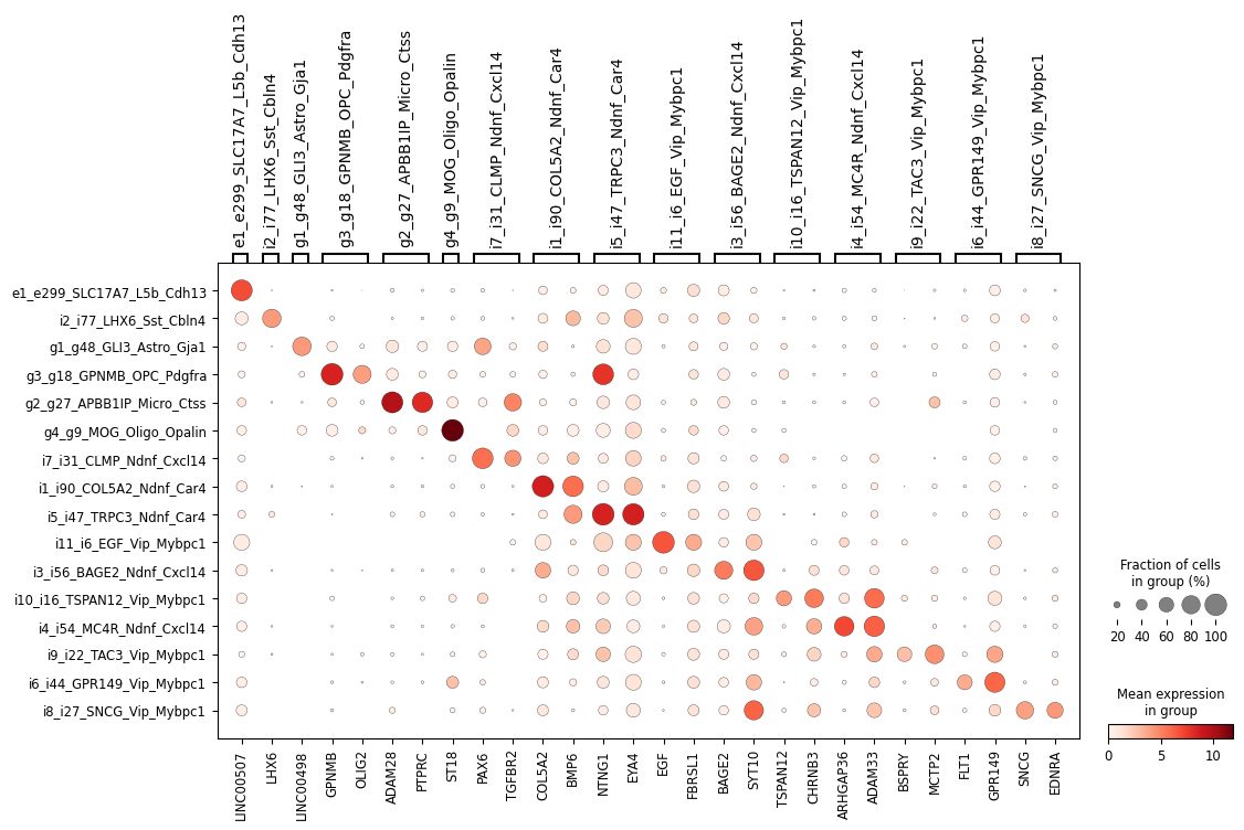
[21]:
ns.pl.dotplot(adata, markers_dict, cluster_header, dendrogram = dendrogram, save = True, output_folder = output_folder, outputfilename_suffix = outputfilename_prefix)
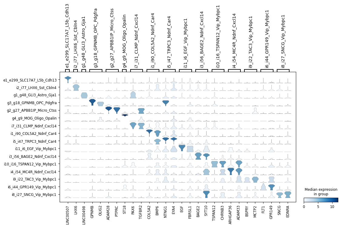
[22]:
ns.pl.stackedviolin(adata, markers_dict, cluster_header, dendrogram = dendrogram, save = True, output_folder = output_folder, outputfilename_suffix = outputfilename_prefix)
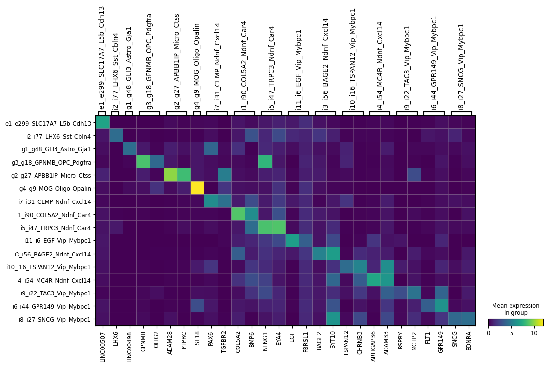
[23]:
ns.pl.matrixplot(adata, markers_dict, cluster_header, dendrogram = dendrogram, save = True, output_folder = output_folder, outputfilename_suffix = outputfilename_prefix)
Plotting classification metrics from NS-Forest results
[24]:
ns.pl.boxplot(results, ["f_score", "precision", "recall", "onTarget"], save = True, output_folder = output_folder, outputfilename_prefix = outputfilename_prefix)
Saving...
 ../outputs_layer1/cluster_boxplot_f_score_precision_recall_onTarget.html
Plotting individual classification metrics
[25]:
ns.pl.boxplot(results, "f_score", save = True, output_folder = output_folder, outputfilename_prefix = outputfilename_prefix)
Saving...
 ../outputs_layer1/cluster_boxplot_f_score.html
Plotting metrics vs clusterSize
[26]:
ns.pl.scatter_w_clusterSize(results, "f_score", save = True, output_folder = output_folder, outputfilename_prefix = outputfilename_prefix)
Saving...
 ../outputs_layer1/cluster_scatter_f_score.html
[27]:
ns.pl.scatter_w_clusterSize(results, "precision", save = True, output_folder = output_folder, outputfilename_prefix = outputfilename_prefix)
Saving...
 ../outputs_layer1/cluster_scatter_precision.html
[28]:
ns.pl.scatter_w_clusterSize(results, "recall", save = True, output_folder = output_folder, outputfilename_prefix = outputfilename_prefix)
Saving...
 ../outputs_layer1/cluster_scatter_recall.html
[29]:
ns.pl.scatter_w_clusterSize(results, "onTarget", save = True, output_folder = output_folder, outputfilename_prefix = outputfilename_prefix)
Saving...
 ../outputs_layer1/cluster_scatter_onTarget.html